T-LoCoH Tips: Analyzing Isopleth Overlap

Summary

This T-LoCoH tip demonstrates how to compute the area of overlap between two sets of isopleths.

Download code in this exercise here.

Background

In T-LoCoH, s is a parameter that controls the degree to which the time difference between two locations is factored into the calculation of their ‘distance’, for the purposes of identifying which points are ‘nearest neighbors’. s=0 corresponds to time being ignored, in which case the distance metric is simply Euclidean distance.

Finding the Area of Overlap Between Two Home Ranges

A number of indices of association have been developed by ecologists for location data¹. The most basic one (but also intuitive) is simply the area of overlap in the home range or core area (often approximated by the 95% and 50% isopleth respectively). In this exercise, we’ll find the area of intersection of the home ranges of two individuals, as computed by T-LoCoH. This same technique could be used to find the area of HR overlap for the same individual during two different time periods, such as wet season and dry season.

Hull-based home range estimators like T-LoCoH compute utilization distributions as a series of nested polygons. So our workflow is essentially to get the correct polygon for each individual, and then find the area of intersection. We’ll be working with home ranges data for two buffalo, pepper and toni, from Kruger National Park in South Africa whose location data are available on MoveBank.org. These datasets have already been analyzed by T-LoCoH and home ranges constructed (see T-LoCoH tutorial for details). Note these datasets are illustrative only, the parameters used have not been cross-checked.

Load T-LoCoH

If you don’t have the T-LoCoH package for R installed, you can get it from (http://tlocoh.r-forge.r-project.org/)

require(tlocoh)

## Loading required package: tlocoh
## Loading required package: sp
## T-LoCoH for R (version 1.18)
## URL: http://tlocoh.r-forge.r-project.org/

Download the hullset for ‘pepper’ the buffalo:

mycon <- url("http://tlocoh.r-forge.r-project.org/pepper.n4571.s0.003.k15.iso.lhs.01.RData")
load(mycon); close(mycon) 

See what it looks like:

summary(pepper.lhs.k15)

## Summary of LoCoH-hullset object: pepper.lhs.k15 
## Created by: T-LoCoH 1.15
## [1] pepper.pts4571.k15.s0.003.kmin0
##       id: pepper
##      pts: 4571
##    dates: 2005-09-16 17:18:00 SAST to 2006-12-31 16:34:00 SAST
## movement: tau=3600 (1hs), vmax=4.827, d.bar=158.4
##    hulls: 4571
##     dups: 9 (offset by 1 map unit)
##     mode: k=15, kmin=0, s=0.003
##  metrics: area, nep, nnn, perim, scg.enc.mean, scg.enc.sd,
##           scg.nn.mean, scg.nn.sd, tspan
##     isos: [1] iso.srt-area.iso-q.h4571.i5
##    other: -none-
##  created: Tue Mar 11 15:34:50 2014

plot(pepper.lhs.k15, iso=T)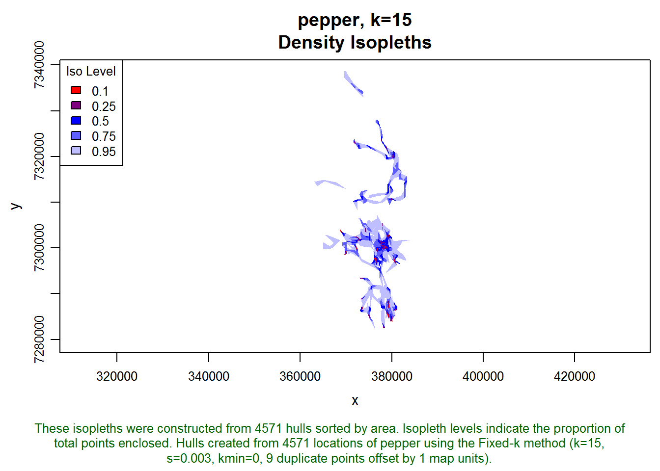

A locoh-hullset object contains a bunch of stuff. We only need the isopleth polygons, which we can extract with the isopleths() function

pepper.isos <- isopleths(pepper.lhs.k15)

The isopleths() function returns a list of SpatialPolygonDataFrame objects, which is how isopleths are saved. In our case, there will only be one list element because pepper only has one set of hulls with one set of isopleths.

class(pepper.isos)

## [1] "list"

names(pepper.isos)

## [1] "pepper.pts4571.k15.s0.003.kmin0_iso.srt-area.iso-q.h4571.i5"

class(pepper.isos[[1]])

## [1] "SpatialPolygonsDataFrame"
## attr(,"package")
## [1] "sp"

Let’s look at the attached dataframe

pepper.isos[[1]]@data

##   iso.level      area edge.len  nep    ptp  hm.val num.hulls
## 1      0.10   1444531    31071  460 0.1006   85056       185
## 2      0.25   6585281    90442 1157 0.2531  171056       544
## 3      0.50  24027295   197715 2288 0.5005  350297      1179
## 4      0.75  62006071   310103 3430 0.7504  658382      2112
## 5      0.95 193837808   367291 4344 0.9503 2342150      3512

Next, we get just the 50th and 95% isopleths for Pepper. We are pulling these out using standard indexing syntax for SpatialPolygonDataFrames (which is very similar to the indexing notation for regular data frames)

pepper.core <- pepper.isos[[1]][ pepper.isos[[1]][["iso.level"]]==0.5, ]
class(pepper.core)

## [1] "SpatialPolygonsDataFrame"
## attr(,"package")
## [1] "sp"

pepper.hr <- pepper.isos[[1]][ pepper.isos[[1]][["iso.level"]]==0.95, ]
class(pepper.hr)

## [1] "SpatialPolygonsDataFrame"
## attr(,"package")
## [1] "sp"

Plot the core and homerange

plot(pepper.hr, border="blue")
plot(pepper.core, border="red", add=T)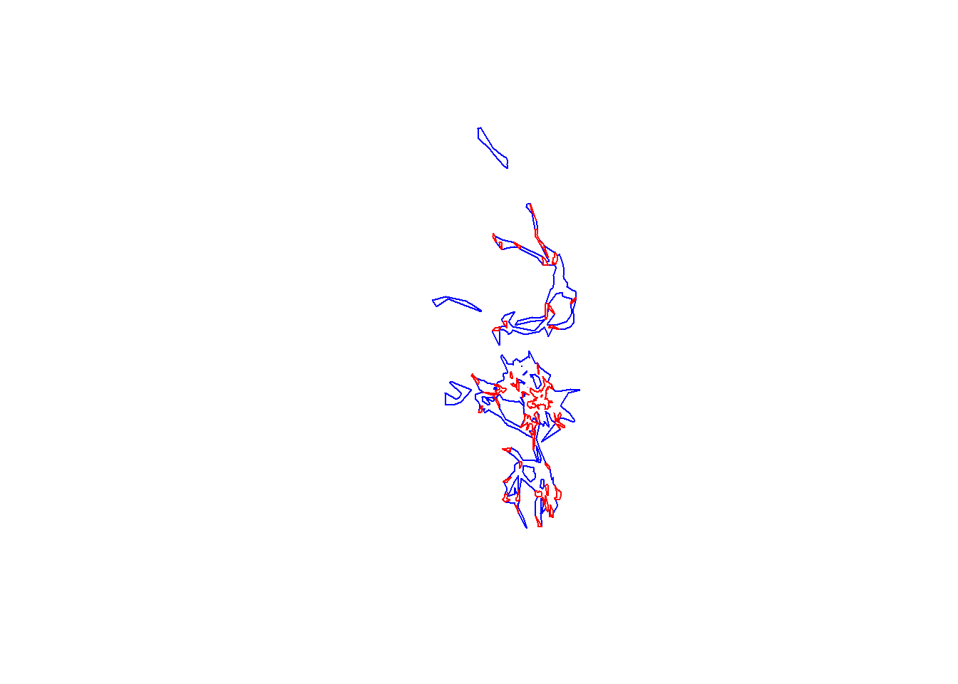

Next, do the same for toni

mycon <- url("http://tlocoh.r-forge.r-project.org/toni.n5775.s0.003.k15.iso.lhs.01.RData")
load(mycon); close(mycon) 
plot(toni.lhs.k15, iso=T)
toni.isos <- isopleths(toni.lhs.k15)
toni.core <- toni.isos[[1]][ toni.isos[[1]][["iso.level"]]==0.5, ]
toni.hr <- toni.isos[[1]][ toni.isos[[1]][["iso.level"]]==0.95, ]
plot(toni.hr, border="green", add=T)
plot(toni.core, border="purple", add=T)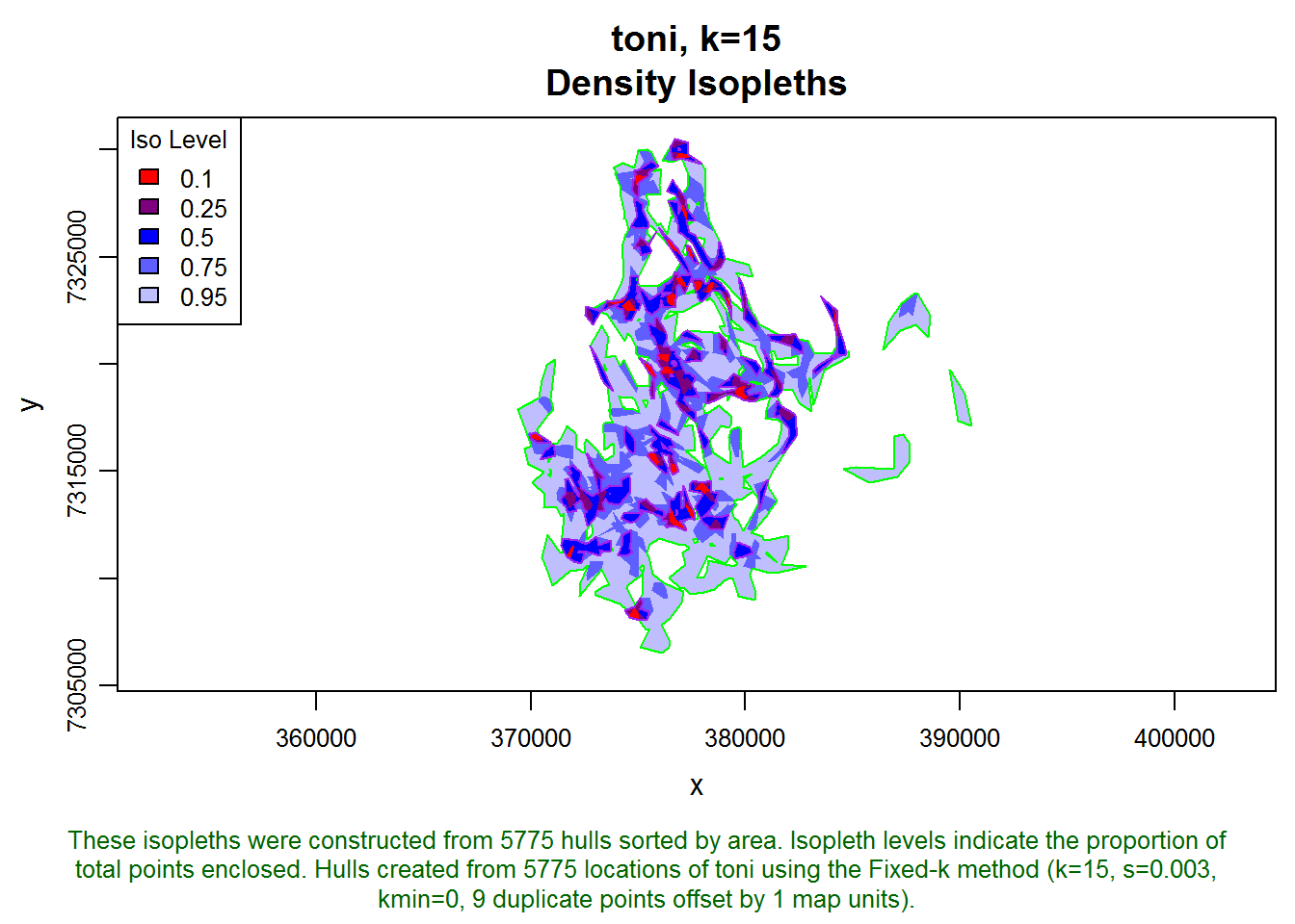

Next, let’s find the intersection between pepper’s core area and toni’s core area. First we’ll overlay them on a fresh plot

plot(pepper.core, border="red")
plot(toni.core, border="purple", add=T)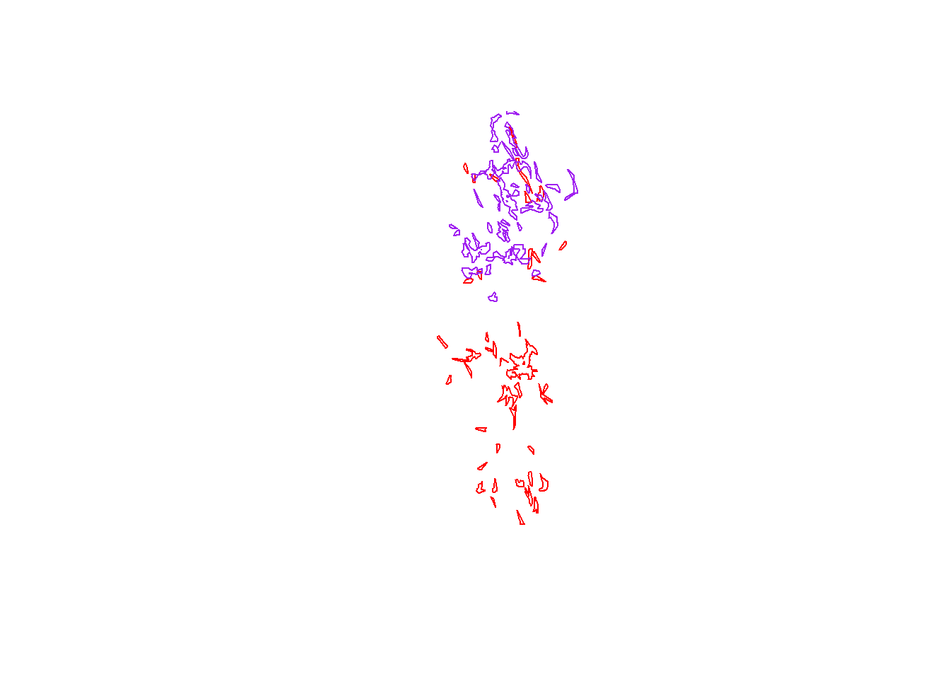

Next, we’ll find the area of intersection of the core areas of Toni and Pepper using a function from the rgeos package:

require(rgeos)

## Loading required package: rgeos
## rgeos version: 0.3-6, (SVN revision 450)
##  GEOS runtime version: 3.4.2-CAPI-1.8.2 r3921 
##  Polygon checking: TRUE

tp.core.common <- gIntersection(pepper.core, toni.core)
class(tp.core.common)

## [1] "SpatialPolygons"
## attr(,"package")
## [1] "sp"

plot(pepper.core, border="red")
plot(toni.core, border="purple", add=T)
plot(tp.core.common, col="brown", add=T)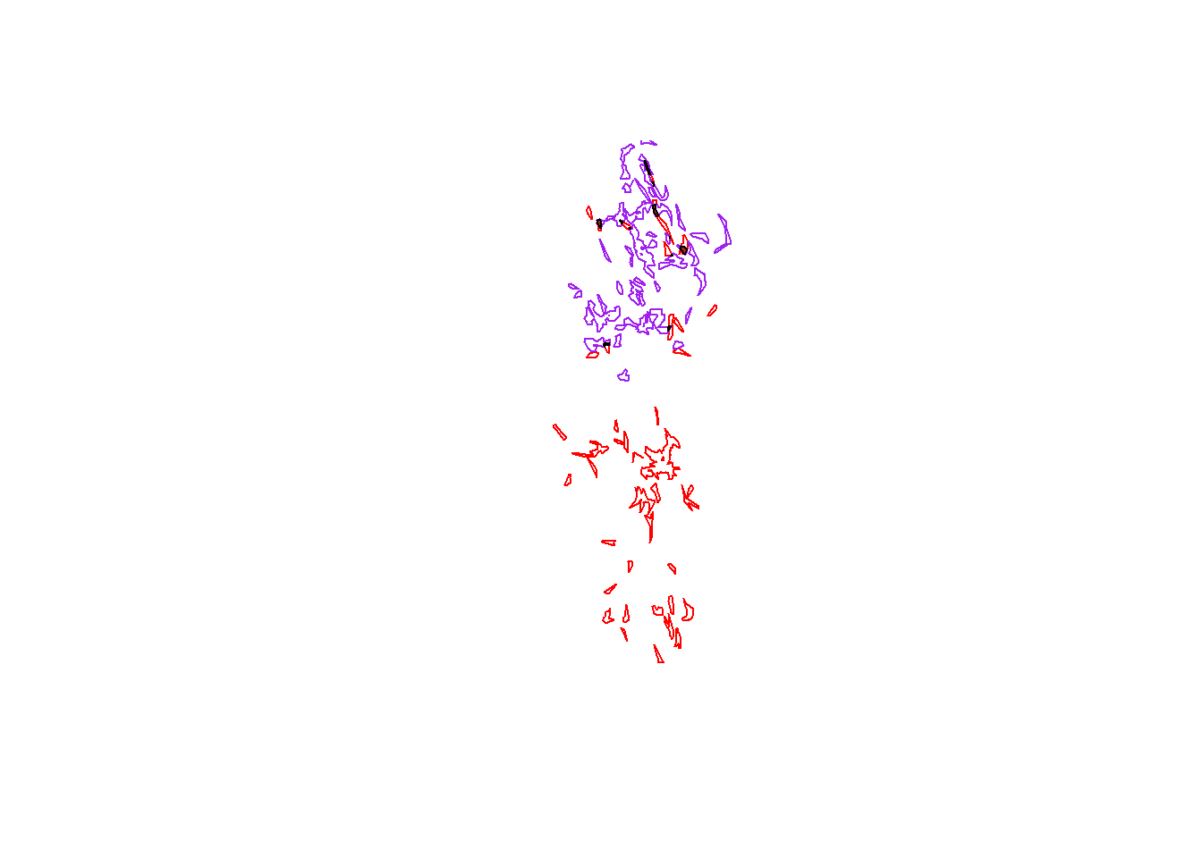

Find the area of intersection of the core areas.

There isn’t a simple built-in function that returns polygon area, but you can easily get it if you know a little bit about the structure of a SpatialPolygons object

tp.core.common@polygons[[1]]@area

## [1] 971545

Next, let’s do the same for the intersection of their home ranges

plot(pepper.hr, border="blue")
plot(toni.hr, border="green", add=T)
tp.hr.common <- gIntersection(pepper.hr, toni.hr)
plot(tp.hr.common, col="brown", add=T)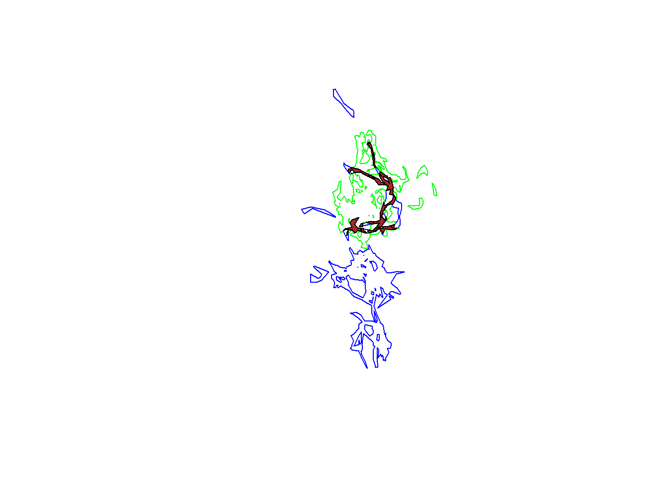

tp.hr.common@polygons[[1]]@area

## [1] 24573476

We see that the area of overlap in the home ranges of toni and pepper is quite a bit larger than the area of overlap of the core areas (which is expected because home ranges are by definition larger than core areas).

This concludes our exercise. A more advanced technique would be to convert the isopleths into a raster probability surface and use the volume of intersection measure of overlap, which we’ll do in another exercise.

---

T-LoCoH Tips. If you find this tip useful, or have feedback or another question on how to use T-LoCoH, please contact the package author.
(c) 2014